Time-Bounded Event-DP Mechanisms
Introduction
To apply differential privacy to a dynamic database, we model it as a stream of items arriving one after the other at each discrete time step. Event-level differential privacy (event-DP) protects the privacy of individual items in a data stream. Time-bounded event-DP mechanisms act on data streams of lengths known ahead of time. In this post, we will learn about a few mechanisms proposed in previous work for privately releasing the number of items in the stream at each time step. We will implement and compare the performance of these mechanisms on toy data streams.
We start by formally defining a data stream and the continual counting query whose answers we want to release. Consider the stream , where an item arrives at time step . Here, is the domain of items, and represents an empty item in case no record is inserted into the stream at time step . Denote the stream with items until a time step using . The maximum possible number of time steps is . The continual counting query is a mapping , such that for each time step , . In other words, maps the current time step to the sum of items that have arrived until then. Now, we want to define a randomized mechanism that releases a continual query mapping that satisfies event-DP for streams up to length . For more details on event-DP, refer to this post.
Mechanisms for Continual Counting
We introduce four event-DP mechanisms proposed by Chan et al. for time-bounded data streams. We consider , i.e., our data stream is a stream of 0s and 1s. This allows us to bound the global sensitivity of the continual counting query: . All mechanisms below provide a pure differential privacy guarantee of for a stream up to length .
Simple Mechanism 1
In this mechanism, we first compute the true count at each step. Then, we add independent Laplace noise with and to the true counts since is the maximum possible length of a data stream. These noisy counts are released. Using basic composition we get a privacy guarantee of . The error of this mechanism is (Chan et al.).
1def simple_mechanism_1(T, epsilon, stream):
2	# compute the true count for each time step
3    private_counts = np.cumsum(stream)
4
5	# add noise to the count at each time step
6    for t in range(1, T + 1):
7        private_counts[t - 1] += laplace_noise(b=(T/epsilon))
8
9    return private_counts
Simple Mechanism 2
In this mechanism, we first add independent Laplace noise with and to each item and release them. Then, we compute the counts using the noisy items. The error of this mechanism is (Chan et al.).
 1def simple_mechanism_2(T, epsilon, stream):
 2	# initialize all counts to 0
 3    private_counts = np.zeros(shape=T)
 4
 5	# add noise to each item
 6    for t in range(1, T + 1):
 7        private_counts[t - 1] = stream[t - 1] + laplace_noise(b=(1/epsilon))
 8
 9	# compute the noisy count for each time step
10    return np.cumsum(private_counts)
Two-Level Mechanism
In this mechanism, we group the items in the stream into blocks of size as they arrive. Over time, each item appears in at most one noisy block sum and at most one noisy item. The noisy count for a time step is computed by adding independent Laplace noise with and to the true block counts and independent Laplace noise (with and again) to the remaining items not part of any block. Using basic composition we get a privacy guarantee of . The error of this mechanism is (Chan et al.).
 1def two_level_mechanism(T, epsilon, stream, B):
 2	# initialize all counts to 0
 3    private_counts = np.zeros(shape=T)
 4
 5    alphas = np.zeros(shape=T)  # for storing noisy items
 6    betas = np.zeros(shape=int(np.floor(T/B)))  # for storing noisy block sums
 7    for t in range(1, T + 1):
 8    	# current noisy item
 9        alphas[t - 1] = stream[t - 1] + laplace_noise(b=(2/epsilon))
10
11        q = int(np.floor(t/B))  # index for new block
12        r = t % B  # check whether a new block sum can be created
13
14        # create a new block sum with the previous B items
15        if r == 0:
16            # compute true sum of items in the new block
17            for i in range(t - B + 1, t + 1):
18                betas[q - 1] += stream[i - 1]
19
20            # store noisy sum of items in the new block
21            betas[q - 1] += laplace_noise(b=(2/epsilon))
22
23        # store private count for current timestep
24        # first sum up all block sums
25        for i in range(q):
26            private_counts[t - 1] += betas[i]
27
28        # then sum up remaining noisy items
29        for i in range(q * B + 1, t + 1):
30            private_counts[t - 1] += alphas[i - 1]
31
32    return private_counts
Binary Mechanism
In this mechanism, we group the items in the stream into blocks of different sizes as they arrive. This grouping depends on the binary representation of the current time step (Chan et al.). The figure below provides the intuition of how the stream is decomposed into a binary interval tree. Each node corresponds to a block of items in an interval. The figure also shows how the mechanism can be implemented using less memory: once a node has been subsumed into a future node, it can be discarded.
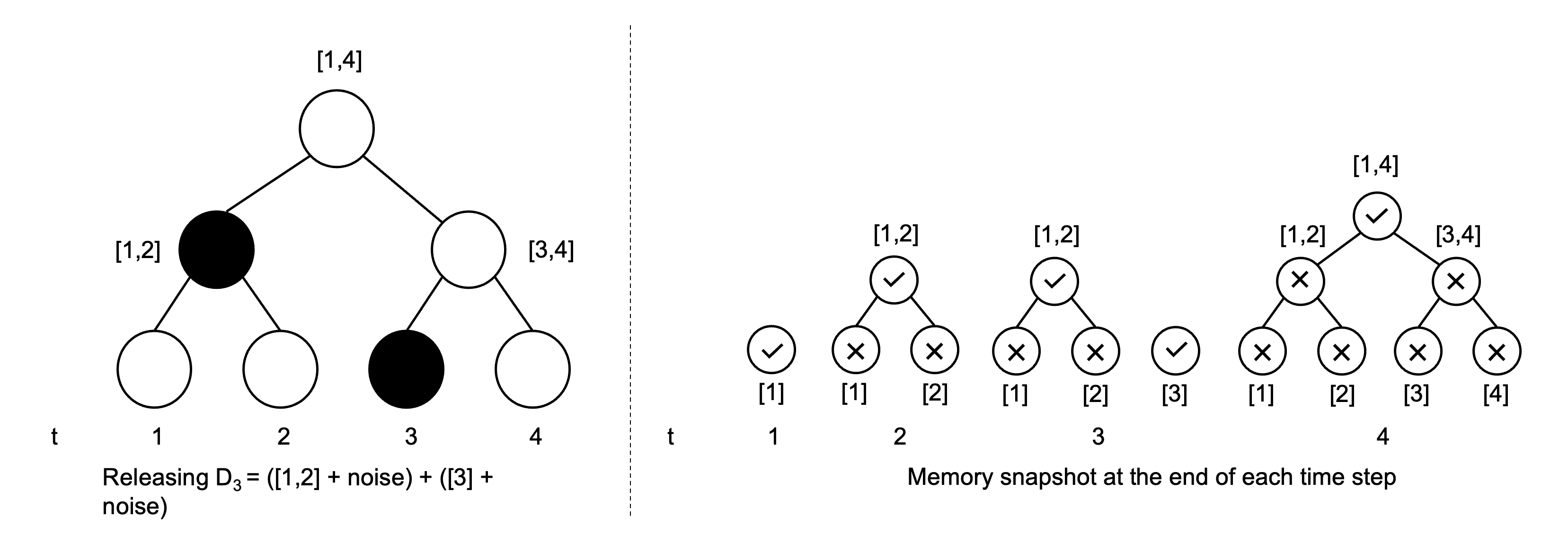
(L) Releasing the noisy count at time step 3 using the Binary Mechanism. (R) Counts stored in memory at the end of each time step.
The count for a particular time step can be obtained by taking the sum of all intervals that make up . Observe that each item appears in at most nodes of the tree over time. The noisy count for a time step is hence computed by adding independent Laplace noise with and to each interval (i.e. node) of . Using basic composition we get a privacy guarantee of . The error of this mechanism is (Chan et al.).
 1def binary_mechanism(T, epsilon, stream):
 2	# initialize all counts to 0
 3    private_counts = np.zeros(shape=T)
 4
 5	# compute number of levels in the binary decomposition tree
 6    log_T = int(np.ceil(np.log2(T)))
 7
 8	# "alpha_i" stores the count for the interval [t - 2^i + 1, t]
 9    alphas = np.zeros(shape=log_T)
10    noisy_alphas = np.zeros(shape=log_T)
11    for t in range(1, T + 1):
12        binary_t = bin(t)[2:]  # time step in binary
13        # get first non-zero least significant bit
14        i = get_first_non_zero_lsb(binary_t)
15
16		# compute "alpha_i" using lower indexed alphas
17        prev_alphas_sum = 0
18        for j in range(0, i):
19            prev_alphas_sum += alphas[j]
20        alphas[i] = prev_alphas_sum + stream[t - 1]
21
22		# reset all lower indexed alphas since "alpha_i"
23		# now contains the sum of their values
24        for j in range(0, i):
25            alphas[j] = 0
26            noisy_alphas[j] = 0
27
28		# add noise to the computed "alpha_i"
29        noisy_alphas[i] = alphas[i] + laplace_noise(b=(np.log2(T)/epsilon))
30
31		# compute the noisy count for the current time step
32		# this is equal to the sum of "alpha_i"s, where "i"s are
33		# the positions of 1s in the binary representation
34		# of the current timestep
35        private_counts[t - 1] = 0
36        rev_binary_digits = list(str(binary_t))[::-1]
37        rev_binary_digits = np.array(rev_binary_digits, dtype=int)
38        idxs = np.where(rev_binary_digits == 1)[0]
39        for j in idxs:
40            private_counts[t - 1] += noisy_alphas[j]
41
42    return private_counts
Performance Comparison
We compare the performance for the four mechanisms at a fixed and streams of length and . We compute the absolute error between the true counts returned by and the counts released by the mechanism over all time steps for measuring performance, i.e., . The results shown below are aggregated over 25 trials.
First, we report the results for streams of length . We can see that the Simple 1 Mechanism has the worst error out of all the mechanisms. Among the other three, Two-Level (with B = 10) performs better at almost every time step. In the initial time steps, both Simple 2 and Two-Level Mechanisms have lesser error than the Binary Mechanism. However, the Binary Mechanism’s error becomes comparable with Two-Level’s as time progresses.
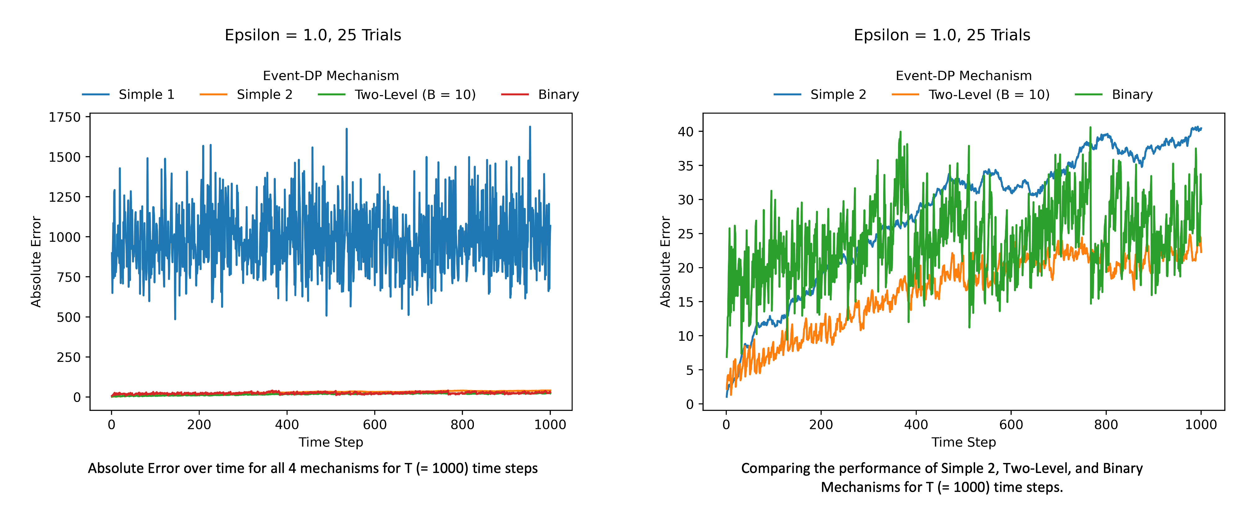
(L) Comparing the performance of 4 mechanisms for T (= 1000) time steps. (R) Since Simple 1 has considerably higher error than the other three, we zoom in to compare Simple 2, Two-Level, and Binary Mechanisms.
Next, we check whether the Binary Mechanism manages to beat the Two-Level Mechanism on increasing the stream length to . The figure below shows this is the case. Around 4000 time steps, the Binary Mechanism starts performing better than the other two mechanisms. However, note that we can improve the performance of the Two-Level Mechanism by picking a better block size. Chan et al. suggest using the block size .
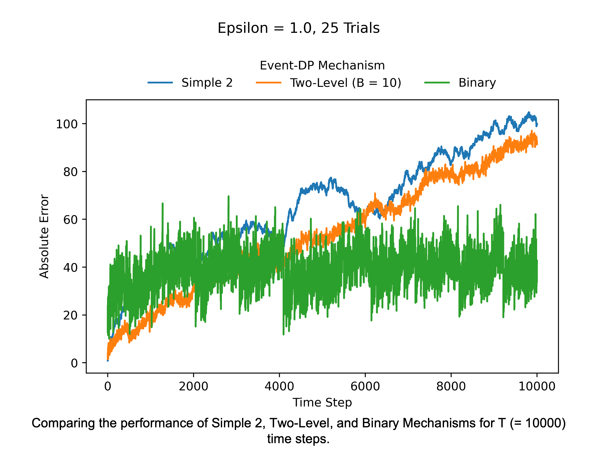
Comparing the performance of Simple 2, Two-Level, and Binary Mechanisms for T (= 10000) time steps. The Binary Mechanism has an almost constant absolute error over time, while the error for Simple 2 and Two-Level significantly increases with time.
The figure below shows how the performance of the Two-Level Mechanism improves as the block size increases. With a fixed stream length, the number of blocks decreases as the size of each block increases. A larger block size implies we can compute the released count for each time step using fewer noisy blocks.
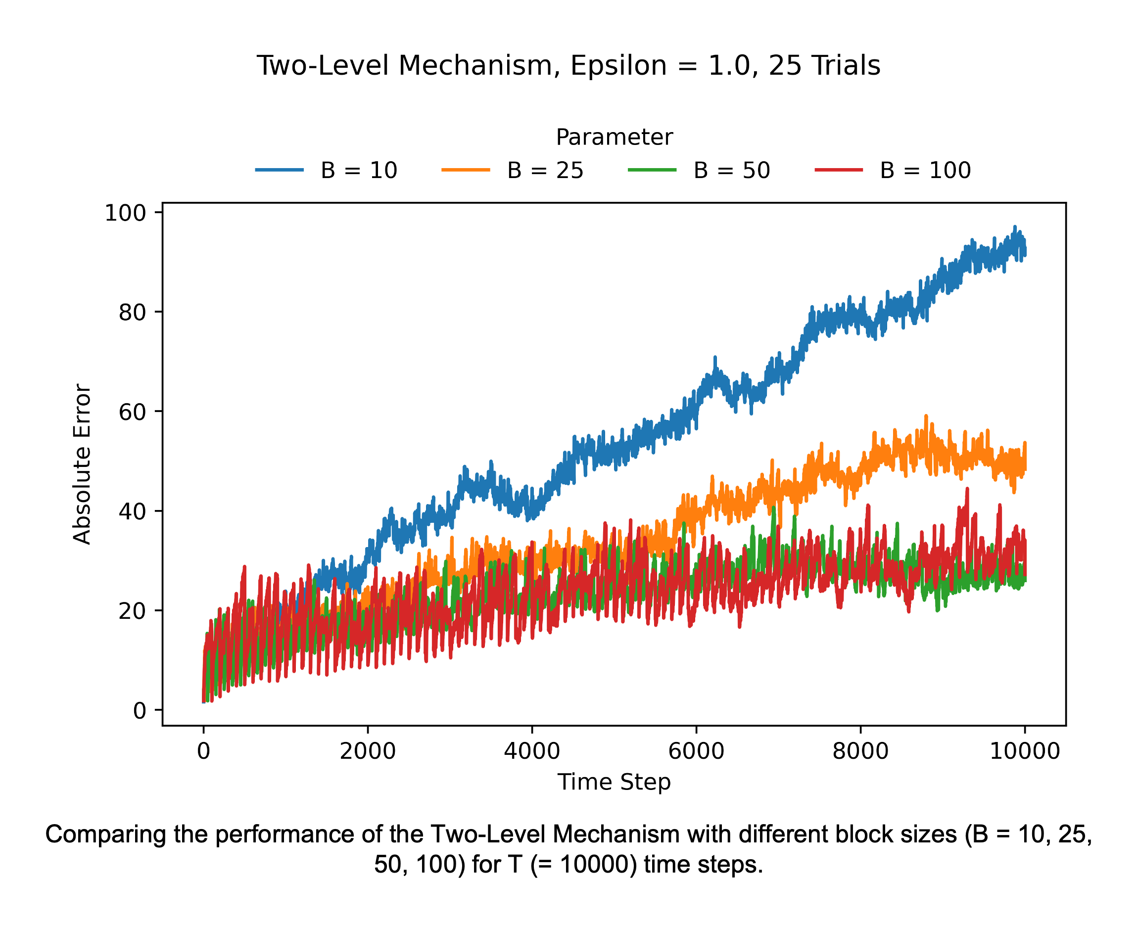
Comparing the performance of the Two-Level Mechanism for different block sizes (B = 10, 25, 50, 100) for T (= 10000) time steps. As the block size increases, the error decreases.
Do these results mean we should prefer the Two-Level Mechanism over the Binary Mechanism? Not always. The Two-Level Mechanism needs us to fix the data stream’s length beforehand, which is not always possible or beneficial in real-world use cases. The advantage of the Binary Mechanism is that we can extend it to support streams of unbounded length. We will explore such mechanisms in a future post.
References
Chan, T. H. H., Shi, E., & Song, D. (2011). Private and continual release of statistics. ACM Transactions on Information and System Security (TISSEC), 14(3), 1-24.